Product Release - Overtime Calculator

Overtime Calculator

Weekly & Bi-Weekly Time Cards

Designed to make entering time into Quick Books easier, this calculator prorates all time over 40 hours for every line item. This makes job costing more accurate and eliminates doing math. 

I recently built this for my own use in my construction business. Because my employees are often on more then one job in a day or have days that aren't 8 hours long, I can't just do 8 hours of regular time and the rest overtime. Quick Books does not calculate overtime. That is why I built this calculator.

Here you can see a sample of what the Time Card looks like. You can change the title to include your business name. My business uses job numbers to track divisions and separate multiple jobs for the same customer.

When using the weekly time sheet in Quick Books, the days are laid out horizontally with the initial of the weekday with the day of the month. Then all times for that day are listed vertically with a total time at the bottom. 

The layout of this spreadsheet makes it easy to tell what day of the week each line is as well as what the totals for each day are. You can see how it is calculating the overtime in the weekday totals.

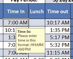
When important, throughout the document instructional boxes will appear to guide you. If their location is not ideal for you, simply click and drag them to where you want them. 

In this calculator lunch is deducted from the total time. So, if your company offers paid lunches, simply do not enter any time in this column. 

The total hours calculates to the minute. Quick Books can handle paychecks being accurate to the minute.  When entering time into Quick Books, use a colon (:) to separate hours and minutes if you are entering to the minute.  If you use a decimal (.) then Quick Books converts that decimals into minutes. So, .5 = 0:30

For the weekly time card, the gross pay details are in the lower left hand corner. Enter the hourly rate you are paying your employee and the overtime rate and gross pay calculate automatically. This is a great double-check before you print the paychecks to ensure your data entry is correct.

You can overwrite the formula here if your overtime is calculated differently. 

 The Bi-Weekly Time Card has a Payroll Report. This summarizes the 2 weeks in the pay period and gives you good totals to compare with Quick Books before printing your paychecks.

Note: Be sure that your time is correct when entered into Excel before entering into Quick Books. Any changes in Excel changes every number as the ratios have changed. If you have already entered into Quick Books before the mistake is found, all of those numbers need updated. 

For my business, I built my payroll report to handle up to 7 employees for 2 weeks and up to 5 workman's comp classifications. If you are interested in having this calculator custom built to match your company, please message me for a quote.

I have provided blank time cards for your employees to fill out that match the design of the weekly time card. Use it if it would be helpful to you.

To see this spreadsheet in action click HERE

For whatever reason Etsy is not allowing Excel files to be uploaded right now, so I have this file for sale on Ebay. You can find it HERE

Thanks for checking it out. If you know someone who could use this, pass it along and don't forget to Follow By Email on the right.

Next week we will be looking at Tools - Styles Group

Nathan
Every Cell = A Calculator!

NERD ALERT!

For those of you who would be interested, I wanted to share a difficulty I came across when developing this product. When Excel calculates time it converts it into a decimal of a day. So, when I started taking my time that was to the full minute and dividing by a percentage of the week, Excel did just that. Only problem was that it was accurate in its math to the second.

It wasn't until I started imputing time into Quick Books that I discovered it was doing this. Because my time format was to the minute, Excel was rounding and my time was off 2 or 3 minutes in every week.

My solution was to use the FLOOR Function to force Excel to stay at full minutes. Now the problem was I had a few minutes that had to be added back in to get to 40 Hours. Using an array SUM inside of an IF function,

I had the spreadsheet add a minute to regular time early in the week until it reached 40 hours and then later in the week to add the minute to overtime. It only adds the minute if that day was short 1 minute after the calculations.

Regardless of if you followed that, know that it is working and that the daily totals help you confirm it is working when you compare it to Quick Books.The same is true of confirming the Gross Pay. Thanks and I will see you next week.

Special Announcement!

Special Announcement!

A Personal Post

This week I am taking a quick break from Excel content to bring you a personal post.  This will be the case in every month that has five Mondays.  This week I want to tell you about a special trip I took and why.

My 10^th anniversary is in September.  Usually this would mean a long weekend away to celebrate with my wife, in September. This year we took that trip in March, because in September Valerie will be 8 months pregnant! This will be our fourth child and a chance at our first daughter.

We just got home from a great weekend at the Chipeta Solar Spring Resort in Ridgway, CO.  I got to go snowboarding while Valerie went window shopping in Telluride. Now, before you accuse me of abandoning my wife and not letting her actual go shopping let me explain.

Because Valerie is 10 weeks pregnant, our midwife and doctor recommended that Valerie not go snowboarding.  So Valerie was able to go explore Telluride while I hit the slopes. Having been married for almost 10 years now, and being graduates (twice) of Dave Ramsey’s Financial Peace University, we discuss big purchases and have a budget for everything else anyways.

With a day to explore the town of Telluride, Valerie rode the free gondola from the ski resort into town. Cash in hand, Valerie walked the streets and was blown away by the outrageous prices of simple items. A sweatshirt hanging on a rack on the sidewalk had a sticker price of $450! We met up for pizza at the base of the mountain and had a good laugh at the ‘inflation’ that has hit these remote mountain towns.

The weekend was filled with beautiful scenic drives and walks up and down main streets of largely deserted towns as this is their slow season between winter and summer. This was very much a picture of our weekend without children that was a wonderfully quiet time before a busy summer of soccer and preparing for our newest member of the family.

Next week the Excel content will resume with a product release of an overtime calculator designed to make data entry into QuickBooks easier. Leave a comment as to which gender you think our baby will be!

Shortcuts - AutoFill Options

Autofill Options

There is a way to exponentially increase your speed in Excel. If you use dates, days of the week, patterns or lots of formulas then AutoFill will transform the way you enter data into Excel.

This post is going to take a lot of pictures to explain the process thoroughly. It will be best demonstrated in this VIDEO if you have 10 minutes to see it in action.

 To start using AutoFill, select the cell or cells you want to copy or use for the start of a pattern. Then put your cursor over the lower right-hand corner of those cells. The cursor will change shape to look like a bold plus symbol.

 Then click and drag that corner down or across to fill those blank cells with your data. A preview of what Excel will put in the last cell is displayed just to the right of the cursor. Because Monday was selected, Excel knows we are looking at days of the week and it is filling the series through Sunday.

 Excel filled the cells with each subsequent day of the week. However, I only want weekdays. Fortunately, this is an option that will be displayed by selecting the down arrow in the tan box to the right of our data.

 By selecting Fill Weekdays in the drop-down menu, cells A7 and A8 change from Saturday and Sunday to Monday and Tuesday. Now every subsequent weekday is displayed for 7 days without typing. This shortcut works over hundreds and thousands of cells, making it one of the most powerful shortcuts in Excel.

 If you want to display every day of the week, this option is called Fill Days.

 When you use AutoFill, it will default to Fill Series or Copy Cells depending on your data type. In this case Fill Days is the same as Fill Series.

 To fill only the formatting and no data, select Fill Formatting Only.

 By using AutoFill, it is easy to copy C2 to D2. By default copying brings the formatting as well.

 To fill the series with just data and not the formatting select Fill Without Formatting.

 AutoFill can be used to more then one row at a time. Select both of the cells you want to use as the beginning of your series. Select the lower right-hand corner and drag to the last cell you want filled.

 Again Excel shows a preview of what the last cell will contain. This is nice to know, so you know how far into the pattern you have gone.

 Not only did Excel fill the days of the week, it also filled in the dates as well using Fill Days.

 Fill Weekdays works on both days of the week and dates.

 Fill Months shows the same date of each subsequent month and the names of the months filled in series.

 Fill Years shows the same date, but changes the year to the next year for every cell selected.

Fun Fact: Excel limits its calculations in relation to time to the year 9999.

 Excel can recognize patterns and will repeat them using AutoFill. To tell Excel to do this enter enough data to represent the pattern and select all of that data.

 Click and drag the AutoFill handle over to where you want the data to stop.  If Excel copied the cells, use the AutoFill Options drop-down menu to change to Fill Series.

Introduction to Absolute Referencing

 Here a simple formula tells Excel to add cells B1 through B5 in cell B8. When this formula is AutoFilled to the 9 cells to the right, the formula changes in each cell to add the cells in the same column as the new formula. This means that the formula in K8 is now =SUM(K1:K5)

 In a formula, the $ symbol locks that portion of the cell reference to keep it from changing. When both the column and the row has a $ symbol, this is called an Absolute Reference. The example above is $A$10. This cell is highlighted yellow and contains the number 10.

 The formula in cell B11 is multiplying B8 and A10. When AutoFilled to the 9 cells to the right, the formula is now multiplying K8 and A10. A10 didn't change because it was an absolute reference. Now every cell that has a formula looking at A10 can be changed by changing the data in cell A10. Here it has changed to 15 and all the formulas updated automatically.

Absolute referencing can be toggled through the options using the F4 key while entering a formula. More detail to come on this in a later tutorial.

Bonus: Customize Status Bar

 At the bottom of the screen in Excel, just below the horizontal slider and just above the taskbar is the Status Bar. Right-click on the status bar to customize it. I recommend turning on all of the quick functions highlighted in red above.

This will give you the ability to analyze your data very quickly without entering formulas. Simply select the data you want to analyze and look at the status bar.

If you have learned something today and want to learn more, follow me by email to receive future posts right to your inbox. I only post once a week, so you won't be flooded with unwanted emails. 

Enjoy your week and God Bless!

Nathan

Every cell = a calculator!

www.etsy.com/shop/ExcelHelpsYou

Introduction to Formulas

Introduction to Formulas - Logical Arguments

Backbones of Formulas

In this post you will learn the symbols that Excel uses to do math. Every cell in Excel is a calculator. If you just type data into a cell, that is what is displayed. If you start with the equals sign (=), then Excel will calculate whatever formula you insert.

A formula is simply anything that requires calculation. A function is a way to tell Excel how to do a calculation within a formula. We will cover functions at a later time.

In Excel every cell has a name or a reference. When a cell is selected, its name is displayed in the Name Box.

Here we can see that cell C3 is selected. Every cell has a default name that is the Column letter followed by the Row number.

When you select a cell, the contents of that cell are displayed in the Formula Bar.

Here we see that cell D4 contains the formula =1+2. The cell displays the result of that formula which is 3. 

By putting a formula in the cell, it became a calculator. It will retain the formula, so that at a later time if you want to know how you got to the result you can still see the calculation. If you used a calculator on your desk to do this calculation, you can't tell if you made a mistake because the data you used would be gone.

This type of formula is static; it will not change until you select the cell and change the formula. 

If you are referencing data in your workbook in your formula, then use cell referencing to make your formula dynamic.

In cell E4 is the formula =C3+C4. This will add the contents of these two cells and display the result. Now when you change the contents of either of those cells, the formula will recalculate.

By changing the contents of cell C3 to 5, the result of the formula =C3+C4 is now 7. This is a very powerful concept to understand.  This can transform a standard spreadsheet into a program that will do the calculations you want.

Here are the symbols for the different logical arguments in Excel as well as sample formulas using those symbols. 

Equals sign

This may seem too simplistic, but I use this a lot. You can put a formula in the cell that you are referencing and only bring the result of that formula into the new cell. This also works on cells that contain text.

Now that you understand the structure of a formula, here is a list of the different symbols you can use to build a formula.

Addition and Subtraction Symbols

The addition symbol is left of backspace and above enter on the number pad.

The subtraction symbol is two keys left of backspace and two keys above enter on the number pad.

Multiplication and Division Symbols

Multiplication is the star symbol above the 8 on your keyboard and above the 9 on the number pad.

Division is the forward slash left of shift and above the 8 on the number pad.

The next two pictures demonstrate comparisons that will yield either True or False.

Less Than and Greater Than Symbols

Less than is the left carrot above comma.

Greater than is the right carrot above period.

Dual Symbol Arguments

These are a combination of two of the above symbols.

Exponent Symbol

This symbol can be found on your keyboard above the number 6. When used in a formula the number after the up carrot is the exponent.

Because I have been repeatedly telling you that every cell is a calculator, I wanted to show you how many cells are in every Excel worksheet. 

The Last Cell in Excel

There are over 17 Billion cells in every Excel worksheet because some people reached the last cell in Excel 2003 and requested more. Microsoft went overboard to help ensure that this problem wouldn't happen again.  

Good luck practicing these new words as you learn the language of Excel.

Click-through to the Vlog version of this episode on YouTube HERE

Next week we will look at the Autofill Shortcut and the Status Bar.

See you next Monday,

Nathan

-Every cell = a calculator!

www.etsy.com/shop/ExcelHelpsYou

Clipboard Group

Clipboard Group

Power hiding in plain sight

Have you ever wondered what the paste symbol is? It is a Clipboard. Most of the time this feature collects data onto the Clipboard in the background, but you can also access the Clipboard on the Ribbon in the Home Tab: Clipboard Group.

By clicking in the lower right-hand corner of the Clipboard Group, you can open the Clipboard Task Pane.

Collection on the Clipboard

Normal copying and pasting does not collect multiple sources of data to be pasted at a later time. Using the Clipboard allows collection of up to 24 different data sources. Data can be collected onto the office Clipboard by Cutting or Copying.

Cutting removes the data from the source. The Cut command looks like a pair of scissors. It is in the Clipboard group and can be pinned to the Quick Access Toolbar (QAT). The shortcut for this command is Ctrl+X or drag-and-drop.

Copying retains the data at the source while collecting the data on the Clipboard.  The Copy command looks like two pieces of paper. It is also in the Clipboard group and can be pinned to the QAT; the shortcut is Crtl+C.

In this example the Clipboard has two data sources collected. The products in this example are fruits and vegetables. Each product needs assigned a type so that you can tell Excel what to do with each type.  

From the Clipboard Task Pane you can click each cell in Column C and then paste one at a time either fruit or vegetable. This would be faster then typing Fruit or Vegetable in each cell, especially if you had 50 different products. 

At the bottom of the Clipboard Task Pane is an options menu that lets you choose when and how the Clipboard acts while it is hidden.

To paste from the Clipboard, either click on the item on the Clipboard, or click to the right of the item in the blue box to open the drop-down menu, then click paste. 

The Paste shortcut Ctrl+V will paste the last data point that was pasted.

To remove an item from the Clipboard, open the drop-down menu for that item and click delete.  If you are done with everything on the Clipboard, then click Clear All at the top of the Clipboard Task Pane.

Drag-and-Drop Cutting

Easily move data around your workbook by drag-and-drop. Select what you would like to move. Click-and-hold on the border of your selection, then drag it to where you want it.

If you want to drag it onto another sheet of your workbook, drag it onto the tab for that sheet and press Alt.

This is what your cursor will look like when you are ready to move an object in Office.

Format Painter

This is a powerful tool that looks like a paintbrush.  It copies a cell's formatting and is then pasted in the next cell or group of cells that are selected.  To paste in multiple different cells, double-click the format painter tool while the cell with the formatting you want is selected.

Because the cells containing Fruit and Vegetable we pasted earlier had thick borders, that formatting pasted as well. By selecting a cell with the formatting we want, in this case cell E17, we can copy just the formatting and not the formula that is displayed in the formula bar.

Click the Format Painter command and select the cells where you want the formatting.

Paste Options

Normal Paste

To paste, select the cell that will be the upper left corner of any data to be pasted.  

Normal pasting brings formatting, formulas, and raw data from the source. It does not adjust column widths.

Paste: No Borders

This option is real straight forward. It does everything normal paste does except it elimanates all borders.

Paste: Keep Source Column Widths

This command can be very helpful if you have taken the time to make the column widths at the source just like you want them.

Paste: Transpose

As a reminder, the columns in Excel are vertical and have letters as headings. The rows are horizontal and have numbers as headings.

Often when organizing data into a blank worksheet, I change my mind halfway through as to how I want to lay out the columns and rows. Paste Transpose will give a quick snapshot of what it will look like to flip your data.  Now the columns and rows have switched. 

Usually you will want to have the categories with the most unique data be your column headings because it is easier to scroll down through your data instead of sideways.

Paste: Values

This paste option allows you to take the result of any formulas you have used to manipulate your data and paste only the values in the destination cells.  Note: Any changes to the cells referenced in the formulas at the source will not cause the destination cells to update, only the values have been pasted.

Paste: Formatting

Very similar to Format Painter, this tool pastes only the formatting.  The destination cells retain the data they contained before the paste. 

The main difference between Format Painter and Paste Formatting is the size of the source data.

With Format Painter the source can be smaller than the destination cells.

With Paste Formatting both the source and destination cells will cover the same number of cells.

Paste: Options

After pasting and before you do anything else, if you don't like how your data pasted you can change which paste option you want.

Open these options by clicking on the Paste Options box that appears in the lower right-hand corner of your data after pasting. Choose the option that works best for you.

To see these tools in action, click-through to the vlog version HERE.

I hope this has been helpful for you. It may take some practice to learn the language of Excel and choose the right tool for the job the first time. 

I'm looking forward to doing more in-depth tutorials. Next week we will look at some basic logical arguments and how to write a formula.

Until then,

Nathan

-Every cell = a calculator!

www.etsy.com/shop/ExcelHelpsYou